
In the entire flow of building a machine learning model, you’re now at the blue-highlighted point.

Suggested Readings
High-dimensional datasets can be overwhelming — too many features make it nearly impossible to see patterns or trends. This is where Principal Component Analysis (PCA) comes in. PCA helps reduce the number of features while keeping the most important information, making it easier to analyze and visualize data.
This guide is divided into two parts: an intuitive introduction to PCA, followed by a practical breakdown using formulas, code, and examples.
Part 1: Intuition Behind PCA
In this section, we’ll explore an intuitive explanation of PCA to solidify the concepts.
Why Do We Need PCA?
When analyzing data with multiple features, it’s easy to get lost in the details. Here’s why PCA is helpful:
- Noise Reduction: With too many features, data may contain a lot of noise, hiding the patterns that matter. PCA increases the signal-to-noise ratio by focusing on the most informative directions.
- Better Performance in Machine Learning: Too many features can slow down models and even hurt accuracy. By reducing features, PCA speeds up training while keeping valuable information.
- Visualization: With high-dimensional data, seeing trends is tough. PCA reduces data to 2D or 3D, making patterns much clearer.
The Core Idea: Capturing the Direction of Greatest Variance
The core idea of PCA is to identify the direction with the largest variance — the axis that best captures how the data is spread out. Why? Because a high variance direction reveals essential patterns, while low variance often reflects redundancy or noise.
Look at the image below. When we project data onto the wrong direction, the points bunch together, making it hard to tell them apart — valuable information is lost. But when we choose the green direction (the one with the largest variance), the points remain well-separated even in reduced dimensions. This shows that more variance means more information preserved.
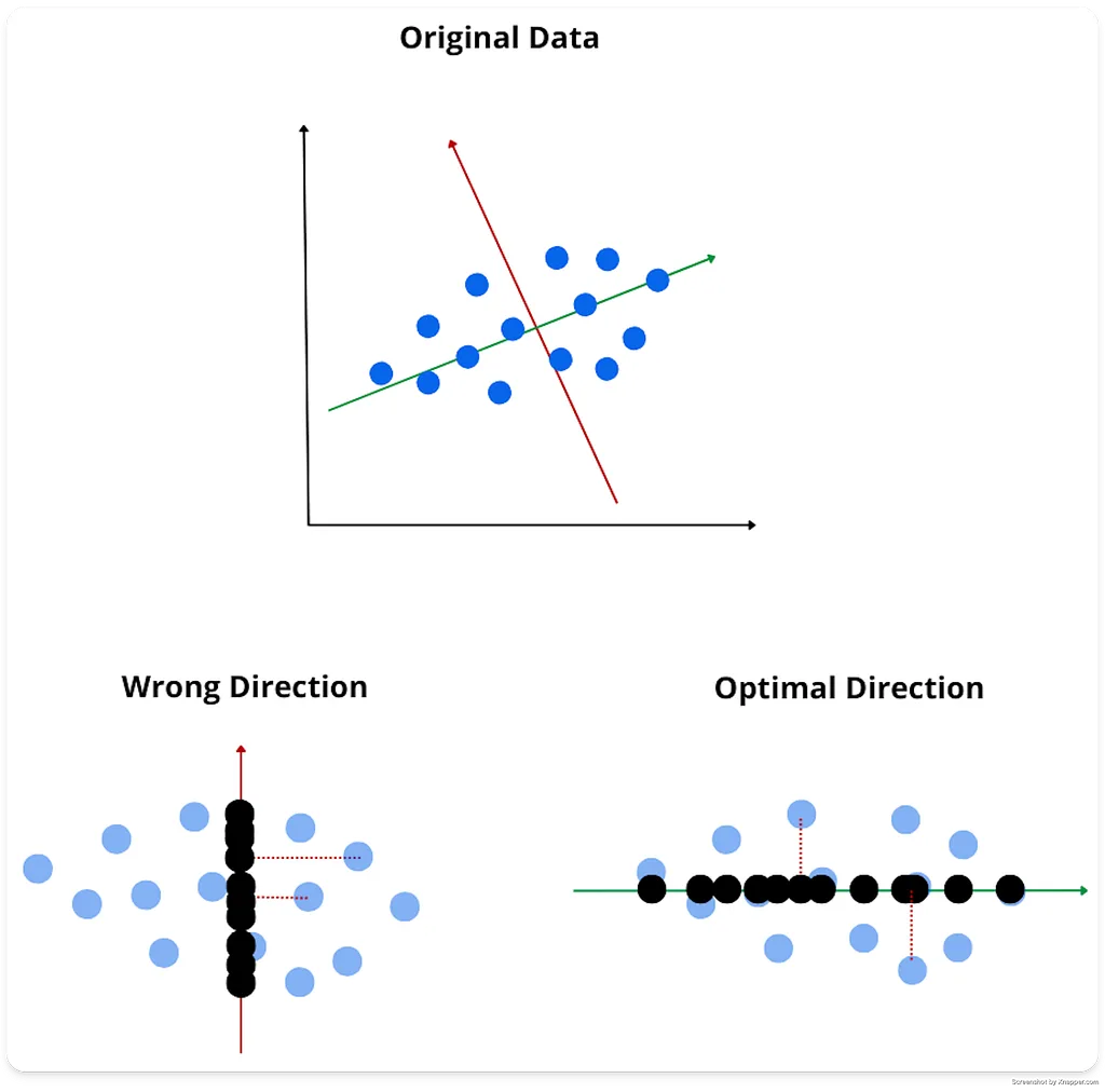
Drawn with Canva Pro
Understanding Principal Components and Variance
Each principal component in PCA represents a new direction in the data, capturing a specific amount of variance, or “spread” in that direction. But why is variance so essential?
Consider a simple classification problem. If all your data points are very close to each other (no variance), it’s nearly impossible to tell them apart — they contain no meaningful information. However, if data points are more spread out (high variance), the differences between them become clearer, providing valuable information for distinguishing patterns.
Intuitive Example:
Imagine trying to classify students based on test scores. If every student scored the exact same on every test, you wouldn’t be able to learn anything useful from that data — there’s no variation to leverage for classification. But if scores vary, the distribution (variance) tells us who might excel or struggle in different areas, enabling us to see unique patterns and make better predictions.
In PCA:
- The first principal component captures the direction of the most variance, retaining the core pattern or “signal” of the data.
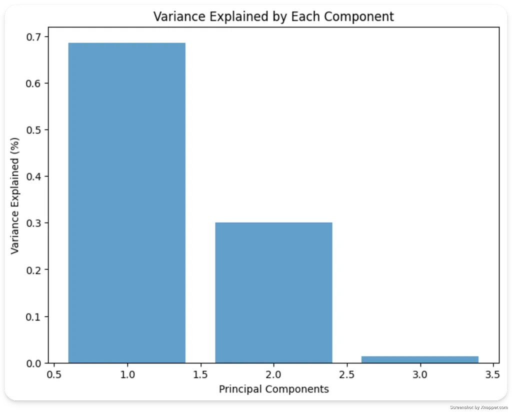
- Subsequent components capture progressively less variance, eventually representing mostly noise.
Scaling Up: From 2D to Higher Dimensions
The reasoning extends easily: PCA can reduce data from higher dimensions, like 50D to 2D, capturing the core patterns and making data easier to analyze. This allows us to work with complex datasets without losing valuable insights and even visualize high-dimensional data in two or three dimensions.
Limitation with Random Forests (RF)
Certain models, like Random Forests (RF), work best when each feature is distinct. Since PCA components are combinations of original features, using them in RF may produce unpredictable results. For RF, it’s generally best to stick to the original features.
Part 2: Practical Computation of PCA
Now we are gonna see PCA under a more practical and technical light.
How PCA Works: Step-by-Step
PCA relies on eigenvectors and eigenvalues, which provide the directions and importance of variance in the data.
1. Center the Data: Subtract the mean from each feature to center data around zero:

Standardizing data is essential before applying PCA to ensure that all features contribute equally. Without it, features with larger scales can dominate the principal components, biasing results and hiding patterns in smaller-scale features.
2. Calculate the Covariance Matrix: This matrix shows how features vary together:

3. Compute Eigenvalues and Eigenvectors: Solve for the eigenvalues λ and eigenvectors (v) of the covariance matrix:

Each eigenvector (v) represents a principal component direction, and its corresponding eigenvalue λ indicates the amount of variance in that direction.
4. Select Principal Components: Sort the eigenvectors by their eigenvalues, in descending order, and select the top ones. This step reduces the number of dimensions while keeping the most significant directions of variance.
5. Transform the Data: Project the original data onto the selected principal components. If we keep k components, the transformation matrix W will contain the k eigenvectors as columns:

Here, X_PCA represents the final, reduced-dimension dataset, transformed onto the new axes defined by the principal components.
Code Example: Applying PCA to Real Data
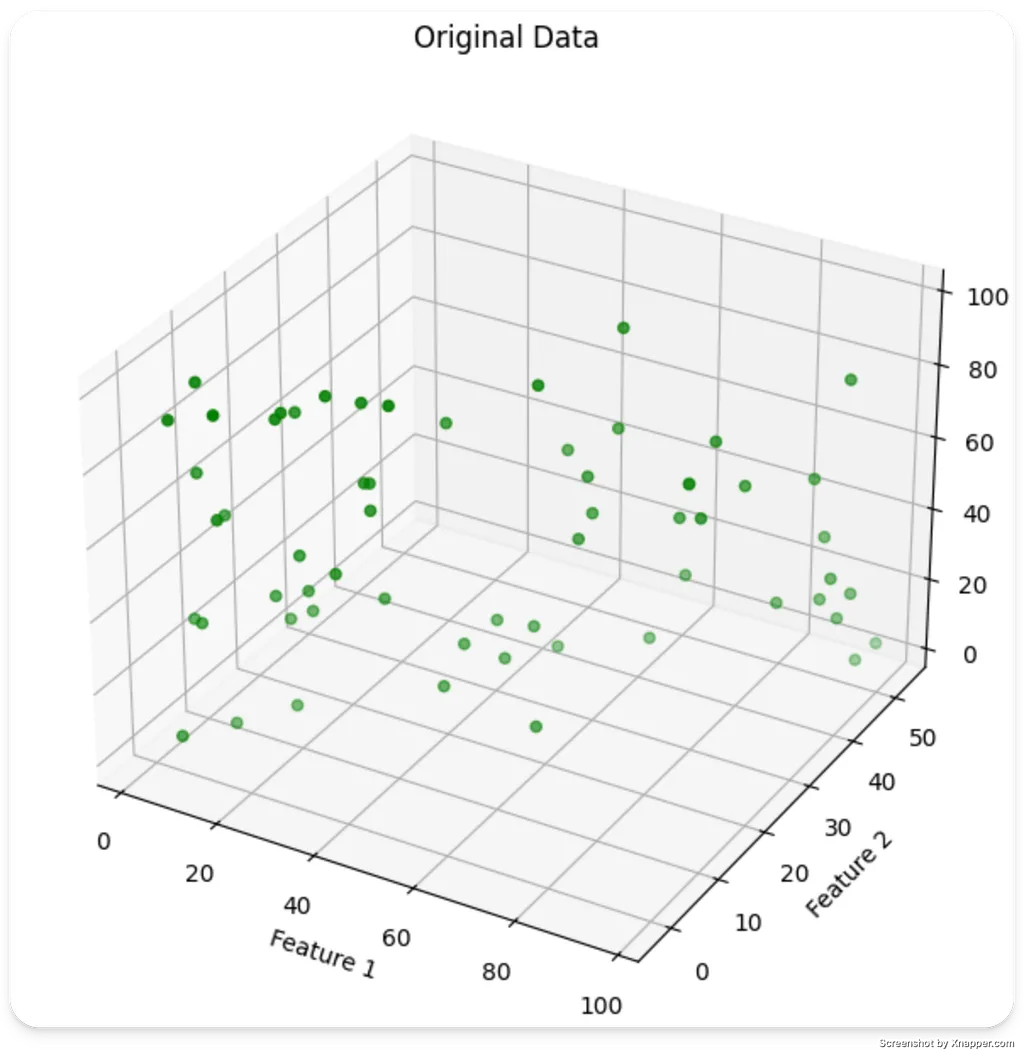
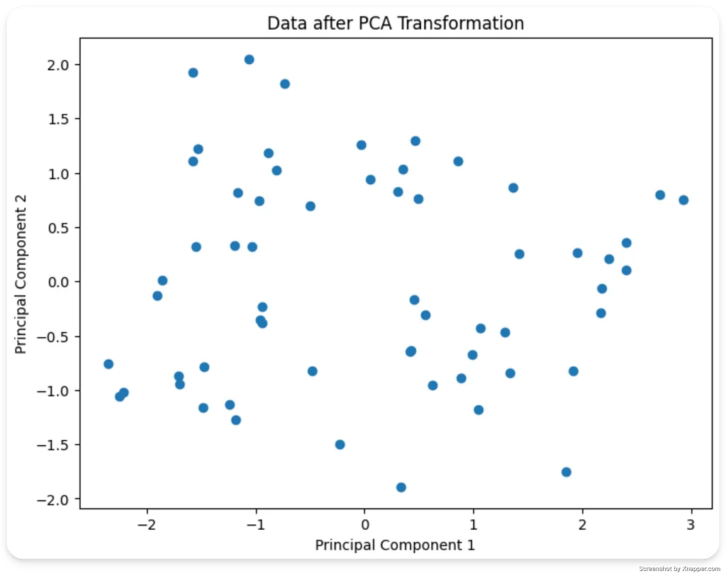
This example shows how PCA transforms data, with the explained variance reducing from one component to the next.
import numpy as npimport pandas as pdimport matplotlib.pyplot as pltfrom sklearn.decomposition import PCAfrom sklearn.preprocessing import StandardScaler# Generate synthetic data with three featuresnp.random.seed(42)feature1 = np.random.rand(60) * 100feature2 = feature1 * 0.5 + np.random.normal(0, 5, 60) # correlated with feature1feature3 = np.random.rand(60) * 100# Combine into a DataFramedata = pd.DataFrame({ 'Feature 1': feature1, 'Feature 2': feature2, 'Feature 3': feature3})# Standardize the datascaler = StandardScaler()data_scaled = scaler.fit_transform(data)# Apply PCA to reduce dimensions to 3pca = PCA(n_components=3)pca_data = pca.fit_transform(data_scaled)# Explained variance for each componentexplained_variance = pca.explained_variance_ratio_# Plot the real datafig = plt.figure(figsize=(12, 6))ax1 = fig.add_subplot(121, projection='3d')ax1.scatter(data['Feature 1'], data['Feature 2'], data['Feature 3'], color='green')ax1.set_xlabel('Feature 1')ax1.set_ylabel('Feature 2')ax1.set_zlabel('Feature 3')ax1.set_title('Original Data')plt.tight_layout()plt.show()# Plot the data in the first two principal componentsplt.figure(figsize=(8, 6))plt.scatter(pca_data[:, 0], pca_data[:, 1])plt.xlabel('Principal Component 1')plt.ylabel('Principal Component 2')plt.title('Data after PCA Transformation')plt.show()# Plot the variance explained by each componentplt.figure(figsize=(8, 6))plt.bar(range(1, 4), explained_variance, alpha=0.7)plt.xlabel('Principal Components')plt.ylabel('Variance Explained (%)')plt.title('Variance Explained by Each Component')plt.show()
Real-World Applications of PCA
- Image Compression: Images often contain thousands of pixels as features. PCA can reduce the dimensionality of these pixels while retaining important details, making it a powerful tool for compressing and storing images efficiently without significant quality loss.
- Genomics: Genomic data can include thousands of genes as features for each sample. PCA helps identify the most critical genes that drive variation, reducing data complexity and aiding in research, such as identifying genes linked to specific diseases.
- Customer Segmentation: In e-commerce or marketing, datasets can have numerous traits for each customer, like age, location, purchase history, and preferences. PCA identifies the most relevant traits for clustering, making segmentation faster and more insightful for targeting and personalization.
- Financial Analysis: In finance, PCA can simplify the analysis of numerous economic indicators, stock prices, or asset features, revealing patterns that drive variation across markets. This helps in portfolio optimization and risk management by focusing on the core components affecting returns.
- Natural Language Processing (NLP): Text data is usually represented as high-dimensional vectors. PCA can reduce the dimensionality of word or document embeddings, allowing NLP models to work with smaller, faster, and less complex inputs without losing key contextual information.
Conclusion
PCA is a versatile tool that makes high-dimensional data more manageable and insightful by focusing on the most informative patterns. By capturing the directions with the highest variance, PCA keeps the essential information while filtering out noise. This simplification is beneficial across various fields, from image processing to genomics and finance, helping in data exploration, efficient model training, and visualization.
Whether you’re preparing data for machine learning or looking to visualize complex datasets, PCA is a fundamental technique in any data scientist’s toolkit.
Download the complete Notebook: PCA.ipynb


